ROS Conductor: A Sawyer Robot Music Conductor

In teams featuring extensive human-robot interaction, there may be inefficiencies in functioning due to operators being uncomfortable with their robotic counterparts. One way to reduce human stigma against robots is to make their motion more humanoid- smoother, more predictive, more adaptive- as has been done by Catie Cuan of Stanford University [1]. Inspired by Catie’s research, my team and I set out to choreograph humanoid motion in the one armed Sawyer robots available to us. We chose to work with the motion of a human orchestra conductor, as the right hand of the conductor, which showcases rhythm and beat changes, can be modeled with a one handed robot. The project uses image processing, audio processing, and kinematic path and velocity planning to drive the desired motion of the robot.

Infrastructure Used:

For the robot, we used Intera’s Sawyer robot, which has one arm. The motion planning was done using ROS’ MoveIt functionality, and the audio input was a microphone processed using ROS’ audio_common library.

Implementation

Motion Planning

In order to start working with a conductor’s motion, we first studied the role of a conductor in an orchestra. Thanks to A Complete Idiot’s Guide to Conducting [2], we found that the role of an orchestra conductor is twofold: To start the performance and establish and maintain a clear and uniform tempo To help the musical quality of the piece (dynamics, rhythm, expression, etc). On account of working with a one armed Sawyer robot, we decided to focus on the rhythm and tempo aspect of conducting, aiming to showcase common motions undertaken by the dominant hand of the conductor. We then looked into the trajectory of the conductor’s baton, and decided to implement two fixed paths recommended by the book for a 2/2 and 4/4 time signature:

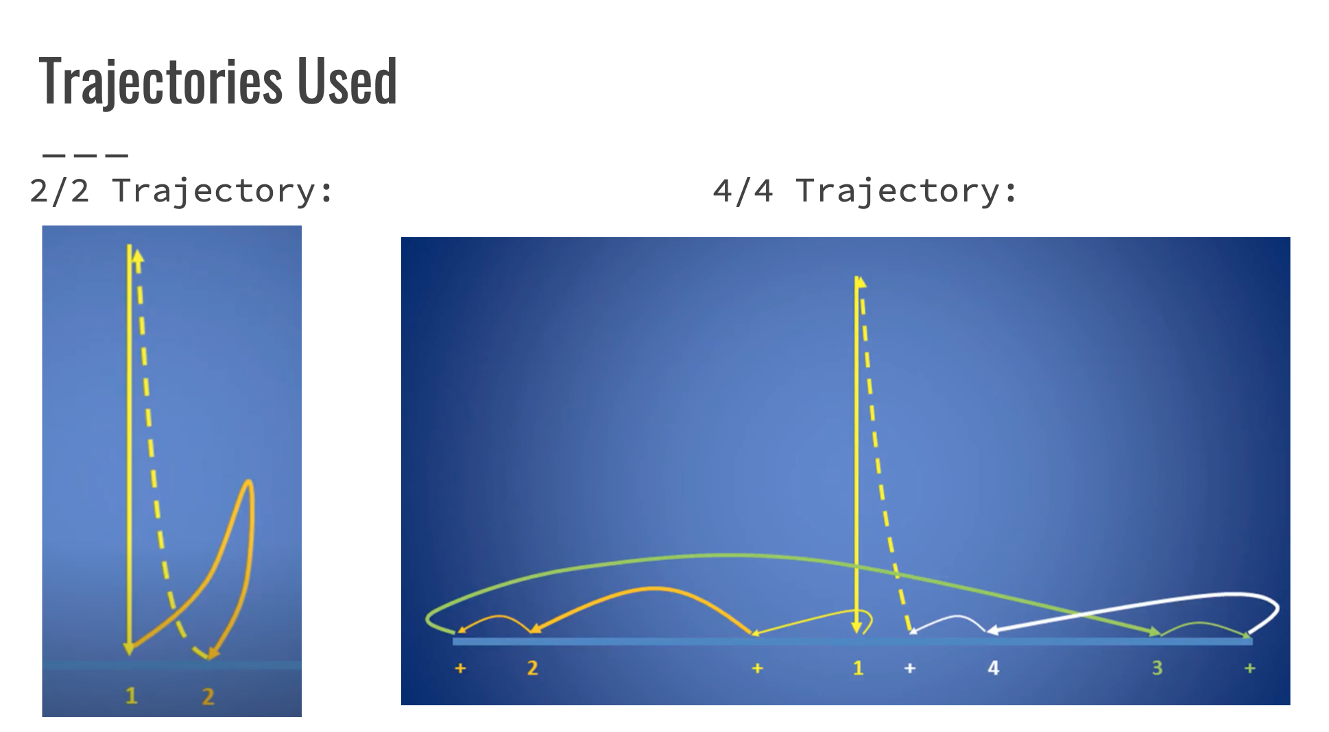
Moreover, we also found that conductors often vary the amplitude and elaborateness of the motion depending on the tempo of the song- higher tempo pieces usually see simpler motions to denote beats and lower tempo pieces can have highly involved beat showcases as seen in figure 1. While there was no official standard for the reduction in amplitude of motion depending on the tempo of the piece, we decided to create our own custom amplitude scaling factor:

Where A is the amplitude, or the distance between the topmost and bottom-most point of a downbeat motion, and BPM is the measured beats per minute of the audio input. We also decided to save multiple trajectories- one with a lot of stops and hand twists and a simpler one in order to switch trajectories depending on the measured BPM.

Once we had the desired trajectories in mind, it was important to become familiar with the workspace of the Sawyer robot. We began by testing our desired upper and lower limits by placing the robot in zero g mode and creating a function called tf_echo meant to mimic the built in ROS tf_echo function in order to get the translation between the stationary and tool frame of the robot.

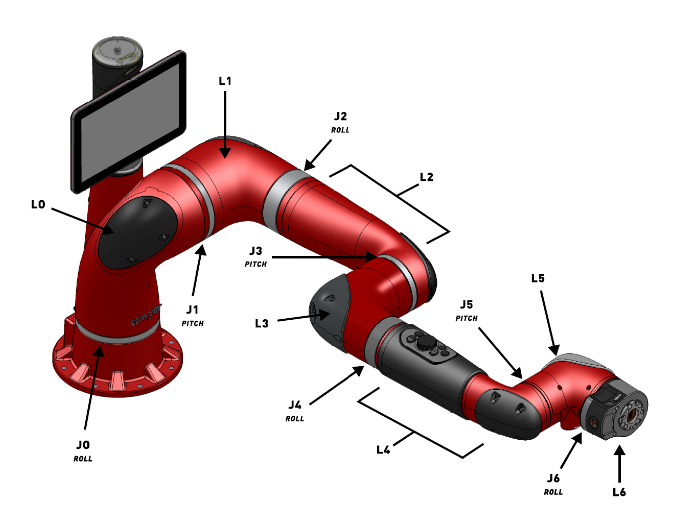
In order to compare the real time TF values to our own calculated values, we used the concept of homogeneous coordinates to find gst(0) from the {S} to the {T} frame. We know that:

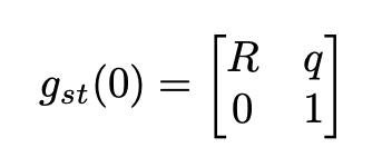
Moreover, by echoing the robot/joint_states topic, we find the required values of q at the given instance of time: 

This allows us to find gst(0) as:

Applying the concept of forward kinematics, we see that

Once again using the robot/joint_state topic of the sawyer robot, we find the necessary thetas and xis at each instance of time, which results in the required gst(theta) value which can then be used for forward and inverse kinematics.

The gst theta was then published onto a separate topic called tf_echo, and the rotation was represented as a quaternion using the 3D rotation to quaternion conversion:

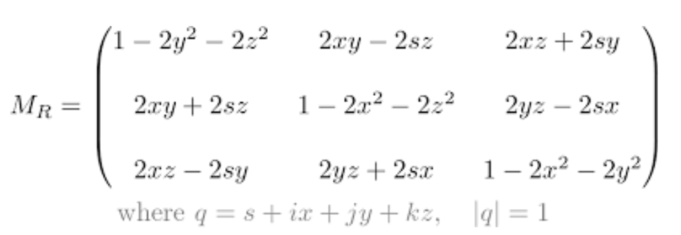
The final message published to tf_echo contained the translation between the {S} and {T} frame as a 3D coordinate and the orientation of the tool frame represented as a quaternion.

Once the tf_echo function was fleshed out, we could get live transformation functions between the end effector and the base of the robot. Then, placing the robot in zero g mode, we took the robot to the highest and lowest point of interest and measured the noted orientation and translation values. We found that the highest point was roughly at [-0.89, 0.835, 0.1] and the lowest point was at [-0.89, 0.2, 0.3]. The x, y, and z axes of the sawyer robot were defined by the blue, red, and green axes as follows:

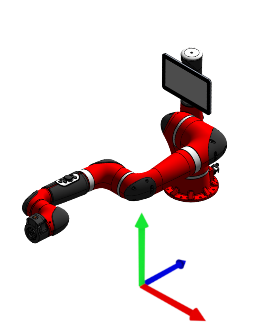
With this information on the end effector position at time t, we went into openCV to extract trajectories from input images for the sawyer robot to follow.

OpenCV and Trajectory Recognition:

In order to extract points along the trajectory for the sawyer arm to follow, we decided to use python’s open camera vision module to process an input JPG image and output translation and rotation in terms of an array of Poses, where each Pose() consists of a translation and orientation. We began by dividing the trajectory into multiple pieces- increasing y direction and decreasing y direction to ease in the sorting of the image array and drawing out those pieces using paint to feed into the image processing node.

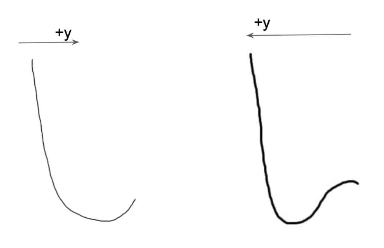
Once the divided image was saved, we implemented a simple thresholding algorithm to filter out pixels that weren’t included in the trajectory. For this, we chose a threshold value between 0 to 70, such that all pixels with intensity within those values would be set to an intensity of 1 and all pixels lying outside those bounds would be set to 0. This ensured that only the pixels lying along the trajectory were noted as the “pixels of interest”, which could be then translated into 3D robot coordinates.

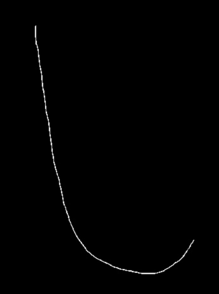
The output image was of dimension [835x1650], with the +z axis pointing downward. In order to align the pixel coordinate z axis and the robot z axis, we implemented a cv.flip() on the image. Further, to scale the pixel coordinates to the robot’s workspace we implemented a simple scaling function as:

Where Delta Z is the vertical distance between two pixel coordinates and Delta Y is the horizontal distance. Scaling those was necessary to expand the image to fit actual 3D measurements mentioned above. We repeated this process for both halves of the trajectory and then vertically concatenated the two arrays together to form a combined point list. The final output was an array of 2D points in the Z-Y plane that the robot arm would pass through while executing the conductor trajectory. However, as the list was over 2000 points long, we were concerned about jerkiness in the robot motion since our chosen planner included a timed stop at every waypoint. This aligned with what we observed as well, and the results of both attempts can be seen in the Links section. Hence, in order to smoothen the motion and also reduce latency in execution, we decided to reduce the >2000 waypoint array to just under 16 critical waypoints that retained the trajectory shape while improving quality of motion. This was done with a simple filtering algorithm that randomly deleted every second element from the image pixels list. Finally, we also eliminated pixels that were less than 5 units close to each other to avoid bumps due to line width capture.

Now that we had a list of discrete x,y,z coordinates for the robot to pass through, we moved on to selecting a planner to create a trajectory through those points. Due to our experience with MoveIt, we decided to use the Cartesian Path Planning functionality of MoveGroupInterface. This allows us to input a list of waypoints expressed in terms of a PoseArray- a list of poses. We also included a table as a path constraint to enable the path planner to navigate around hard obstacles.

The output from the cartesian planning algorithm was a RobotTrajectory message which contained joint angles and velocities at each given waypoint.

Node Structure and testing implementation:

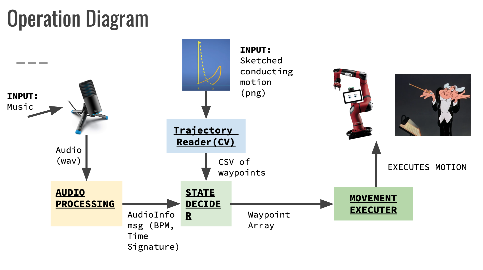
We wanted our implementation to be rapidly iterable, hence we decided to split our code into three nodes- audio processing, image recognition and state decision, and movement execution. The audio processing node took audio input, converted it into a .WAV file, and used pattern recognition to identify the salient BPM of the audio file. We also decided to map a “high” BPM- defined above ~150 BPM to a 2/2 motion, since that was less elaborate and required less time to complete. A “low” BPM was mapped to the 4/4 motion, which had multiple stops and would require longer to execute fully. The image processing was all done beforehand, since the trajectory for a particular time signature wouldn’t change as the motion was happening, and we wanted to avoid latency due to time lost during image processing. The state decider node took the calculated trajectory waypoints as a CSV file and mapped them to a dictionary where the keys were the “low” or “high” signal of the BPM. The state decider served as both a publisher and subscriber node and published the calculated PoseArray of waypoints onto the state_info topic, which was subscribed to by the movement executor node. The movement executor node took in the list of waypoints, calculated the cartesian path, and finally executed the plan using the move group execute() function.

Results and Improvements:

Upon testing the cartesian path planner, we realised that despite reducing the number of waypoints, the trajectory was jerkier than expected since the time stop at every waypoint was quite significant. This was especially noticeable for the 4/4 trajectory. Moreover, the velocity of the robot couldn't be scaled with the max_velocity and max_acceleration scaling factors provided by MoveIt. Upon further research, we realised that this could be solved by using a different planner- particularly, the Pilz Industrial Motion Planner which allows the user to specify a bend radius used to pass each waypoint and the velocity during trajectory execution. This would allow us to get a real time beat on beat time signature motion as required.

We plan on expanding on the current functionality of the robot by incorporating a real time and smoothening portion into our implementation, as well as the variable amplitude scaling dependent on BPM. Now that we know how to provide multiple points for a robot to move through, the next step is syncing the conducting motion of the robot to the actual beat input, which will be done by publishing the time stamp at which a beat occurs in a song and executing a timed motion based on a calculated latency in data transmission. We believe that the implementation of the Pilz Industrial Motion Planner will allow us the desired velocity control to ensure that our trajectory is executing within the specified time frame that it takes to denote a time signature (for example 2 seconds for a 2/2 time signature). We also plan on using mercator projections to map the 2D points of the robot end effector to its spherical workspace, which we believe will result in a smoother motion with less loss of efficiency in unnecessary joint turns.

Links and References

Github Repository of Code
https://www.scientificamerican.com/article/dancing-with-robots/
Move it messages ROS documentation
Geometry messages ROS documentation

Contributors

Motion Planning and CV: Nayesha Gandotra and Ryan Ho
Music and BPM Recognition: Bob Ni and James Liu